 |
You should always perform initial processing in Topspin to verify that experiments worked. Once you are certain that data is OK, processing in MNova gives better quantitative results and overal presentation. To process in MNova, follow the steps below.
1. Open a DOSY data by dragging the Bruker Expno with the dataset into the open MNova window on a new page (Cmd-M to make a new page in the document).
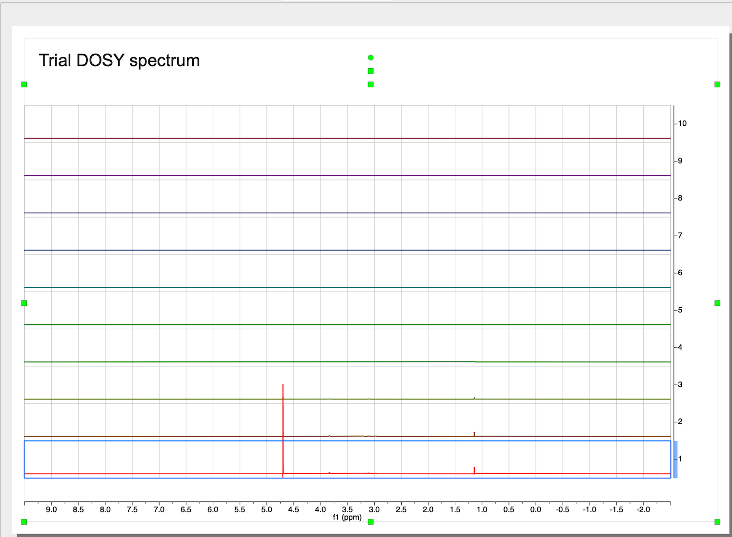
2. DOSY dataset opens in a stacked mode with the trace acquired with a smallest gradient on the bottom. Click inside of the stacked spectrum and pull down on a green square to adjust it size from the top. Give a name to the page.
3. Next step is to process the series of DOSY spectra contained in the dataset. Click inside the bottom spectrum to make it selected.

4. Next, find the tab called called "STACK" on top of the ribbon and click "Stacked", "Mode", "Active Spectrum"
5. Now we have only one spectrum of the stack shown on the screen: the first trace with the smallest gradient and largest signal.
6. The manual phase and baseline corrections are described in the Episode 4 of my series "Data Processing in MNova NMR" https://pydio.campus.nd.edu/docs/doku.php?id=mnova_data_processing
7. First, perform a phase correction only.
This is a starting dataset:
Make sure the baseline before the peaks continues into it baseline after the peaks. Ignore the distortion of the very intense peak of residual water.
10. Inspect the full diffusion series now. Go to STACK tab, select "Stacked", Mode:Stacked.
Roll mouse up. The second trace phase is not good - baseline correction may fail.
11. To adjust 2nd trace individually we need to select it and isolate from others otherwise our changes will distort other spectra in the stack. Click STACK:Stacked:Stacked Items Table. A table with all traces opens.
Return to the spectrum view and click on the bad spectrum to select it. The spectrum name and numbers in its line in the table became bold, which means it is the selected spectrum.
Uncheck the box with a "Pushpin" column.
Click arrow down on the button "Select" and choose "invert selection".
Now the 2nd spectrum is the only one that will be affected by adjustments.
12. Select STACK:Stacked:Mode:Active Spectrum
manually adjust the phase of the spectrum:
Return to Mode:Stacked. All other spectra are unaffected!
NOTE: You may remain in the Active Spectrum mode and switch the current spectrum you are working on by unchecking previous, checking the new one and double-clicking on its line in the Stacked Items Table
13. Select all spectra again: Visit Stacked Items Table and choose Select:Select All.
14. All spectra have good phases. We may proceed with a baseline correction. Similar as we did for the phase correction above: make the first spectrum active.
Baseline is offset into negative values. To correct, first zoom in to leave out distorted ends of the spectrum.
Choose Processing tab in NMR, click on arrow down in Auto Baseline Correction, and select Baseline Correction. Select "Polynomial Fit", uncheck "Autodetect" option, check "Run on region" option and "Get Region from Zoom". Now move the slider until you see a satisfactory shape of the correction curve (blue line) passing through the baseline regions of the spectrum.
Click OK: Baseline is corrected and shifted to zero.
More advanced method: Multipoint Baseline Correction:
To do multipoint correction:
- click Pick Point and carefully click through all baseline regions between peaks. You do no need to point at baseline with a cursor - just position it at the ppm that is a baseline.
- Save your points by clicking Save button and place the CSV file next to your datasets
- Click Preview to check the result. Ignore the ends of the baseline - you will cut them out
- Click Apply
- Check the results of other spectra
- Cut the extreme ends of the spectra to remove the artifact (steps). Use Cut tool (X)
NOTE: Sometimes, MNova glitches and does NOT update the baseline correction result. Exit and relaunch!
15. Same parameters were automatically applied to other spectra. Switch to Mode: Stacked:
Roll mouse wheel to zoom and check for problems in other spectra
Two spectra close to the end of the series (top) have a problem with baseline correction on the right.
16. We need to adjust baseline only for the affected two spectra. Isolate them as done previously: click on one to select, uncheck "Pin" column
invert selection
and make selected spectrum "Active" (Mode:Active Spectrum):
This function is a little glitchy, which is frustrating, but you may still succeed. If correction preview (blue line) does not go well through the baseline portions, play with parameters: switch out of Polynomial Fit method and select it again, and uncheck and check back on region, move the slider. Visually choose what makes a reasonable correction curve.
Switch back to Mode:Stacked and verify that adjustments to both traces were good. You may as well fix the two spectra one by one.
Go to Stacked Items Table and Select:Select All to make all spectra available for analysis.
The dataset is ready for the diffusion coefficient fitting.
18. First, we check parameters of DOSY experiment. Select View:Tables.
Check "Arrayed Data" and click OK.
See if your large delta is equal to D20 parameter in the Bruker DOSY setup and the lowercase delta is 2x p30 pulse length (in seconds; for bi-polar gradient experiment like BPP-STE).
NOTE: You may look them directly in the dataset. Open a file acqu in text editor and search for ##$D=. These are all delays numbered from 0. D20 will be the 21st value in seconds. Then search for ##$P= and look up 31st value for p30, in microseconds.
19. Simple and quick analysis of DOSY series may be done to create a traditional DOSY presentation. Click on the DOSY spectrum series, select STACK:Stacked:DOSY/ROSY Transform. Select Bayesian, and hit OK.
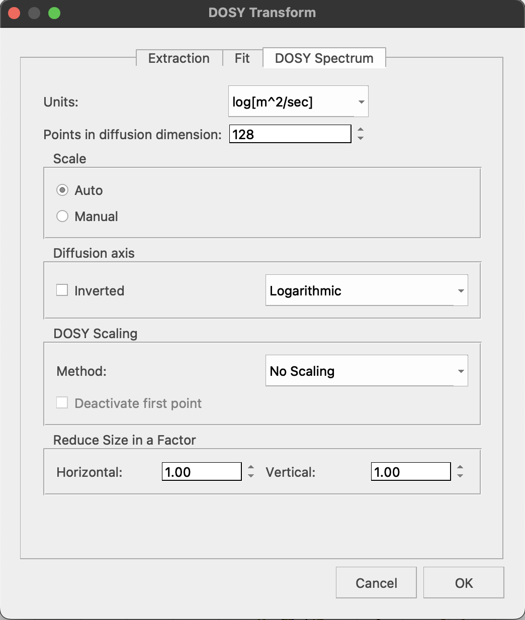
In newer MNova: Switch to Fit tab, select Bayesian, switch to DOSY Spectrum and hit OK
This however will only be successful if you have a spectrum where peaks of different compounds do not overlap. Since it is not the case most of the time, I prefer peak-by-peak analysis instead.
20. Pick peaks for analysis. You need to select peaks that are NOT overlapped with others! Make first spectrum Active. Use Analysis: Peak Picking: Peak by Peak option (K). Make sure you pick buffer components and water too because they serve as an internal reference!
21. Return to Mode:Stacked and roll the mouse wheel to increase intensity. Zoom and verify that peak positions remain the same in all spectra.
No peak drifts in my dataset! Proceed...
NOTE: If there was a slow gradual drift, the "Autocorrect peak positions" option will be needed (see below).
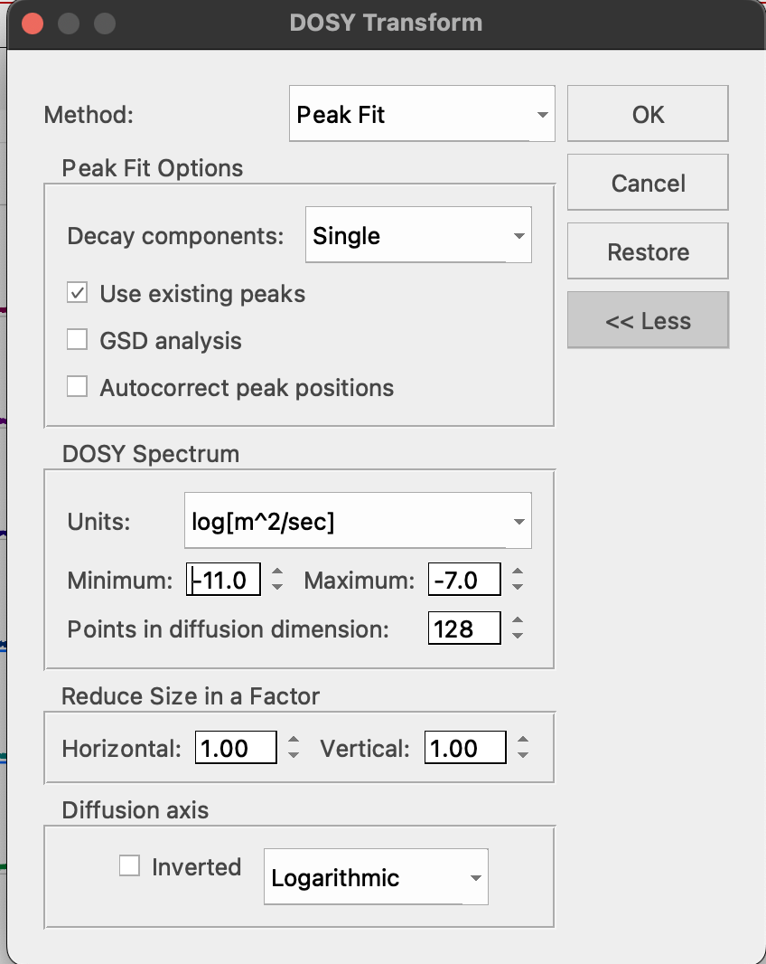
22. Click Stacked: DOSY/ROSY and select Method: Peak Fit. (left - old MNova, right - New MNova)


You may select any units but if you use "log(m2/s)", it will match default units of the Topspin DOSY transform so they will be easier to relate.
Important: do NOT click Diffusion Axis: Inverted! It glitches and will destroy the result. Instead, just keep in mind the Y axis is inverted relatively to Topspin DOSY transform.
If peak positions were drifting, check "Autocorrect peak positions".
Click OK to run the fitting.
23. Peaks with diffusion coeffients are displayed. You may zoom in and roll the mouse to see a simulated DOSY plot. The line width in proton dimension is related the width of the original signals, while width in the diffusion coefficient dimension is related to the fitting error.
Peak list with values of D may be obtained through View: Tables: NMR: Peaks.
This table may be copied to clipboard and pasted into Excel for analysis.
Column f1(DOSY) contains log10(D).
25. If you are interested in detection of changes in diffusion coefficients, overlaying 2D plots (obtained at the SAME temperature!) makes changes visual, as in this example:
Overlap of reference signals like water and buffer salts serves as internal measure of accuracy of this comparison.
Important notes
- Computed values of a diffusion coefficient will be always off from real numbers by a fixed amount because calibration of NMR probe gradient coil is not perfect. To make a correction, find a literature value for the diffusion coefficient for water or other compound in your tube at your temperature in the solvent with identical visocity.
- To correct all diffusion coefficients using a reference value:
- Log10(D, corrected) = Log10(D, observed) + [ log10(D, reference compound, from literature) - log10(D, reference compound, observed)]
or
- D(corrected) = D(observed) * [D(reference compound, from literature)/D(reference compound, observed)]
- In the first approximation, you may use this reference value: D of residual H2O in pure D2O at 298K is 1.902e-9 m2/s (in Claridge, p317 in 2nd and p397 in 3rd editions), which corresponds to log10(D) = -8.72
- You can ONLY expect your measurement give you accurate diffusion coefficient if your molecule is present in only ONE form with one size/aggregation state. If you have monomers, dimers, trimers, etc. and chemical shifts are the same that is peaks are exactly overlapped, the D value will be some sort of weighted average. It will still reflect on the aggregation states but will not be interpretable directly. Fitting to obtain of more than one diffusion coefficient from a single peak (decay curve) will ONLY be reliable if your diffusion constants differ by at least of factor of ten. However, amount of signal from the heavy species will be minimal therefore this case is not practical either.
Literature:
High-Resolution NMR Techniques in Organic Chemistry, 3rd Edition, by Timothy D.W. Claridge. Elsevier Science (May 27, 2016), ISBN-10 : 0080999867, ISBN-13 : 978-0080999869
 |